Inspect Agents Performances

Necessary imports

from copy import deepcopy
import toolz
import seaborn as sns
import matplotlib
import matplotlib.pyplot as plt
from myst_nb import glue

from colosseum import config
from colosseum.agent.mdp_models.bayesian_models import RewardsConjugateModel
from colosseum.agent.mdp_models.bayesian_models import TransitionsConjugateModel
from colosseum.experiment.agent_mdp_interaction import MDPLoop
from colosseum.agent.agents.episodic import QLearningEpisodic, PSRLEpisodic
from colosseum.mdp.river_swim import RiverSwimEpisodic
from colosseum.utils import make_mdp_spec
from colosseum.utils.acme.in_memory_logger import InMemoryLogger
from colosseum.analysis.visualization import plot_MDP_graph
from colosseum.analysis.visualization import plot_MCGraph

sns.set_theme()
config.enable_verbose_logging()

\(\texttt{Colosseum}\) implements several performance indicators. After describing them, we report the agent classes and the environment classes implemented in the package. Then we’ll compare the performances of two agents in the same environment, and the performances of an agent across different MDPs. When comparing across different environments, normalized versions of the indicators should be used to account for transition kernel and reward kernel differences.

Indicators

Reward-based indicators
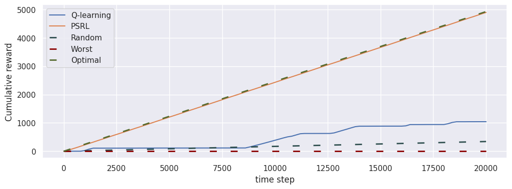
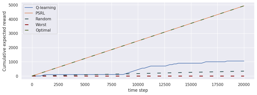
The \(\texttt{cumulative_reward}\) measures the empirical cumulative reward the agent obtains while interacting with the MDP. The \(\texttt{cumulative_expected_reward}\) indicator measures the expected average reward for the agent’s best policy at fixed intervals and cumulates them.
Regret-based indicators
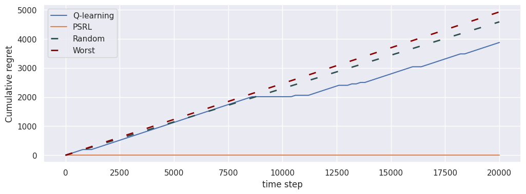
The \(\texttt{cumulative_regret}\) computes the expected regret for the agent’s best policy at a fixed interval and cumulates them.
Baseline indicators
The \(\texttt{cumulative_expected_reward}\) and the \(\texttt{cumulative_regret}\) indicators are also available for the uniformly randomly acting policy, the optimal policy, and the worst-performing policy.
Computation cost
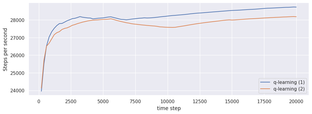
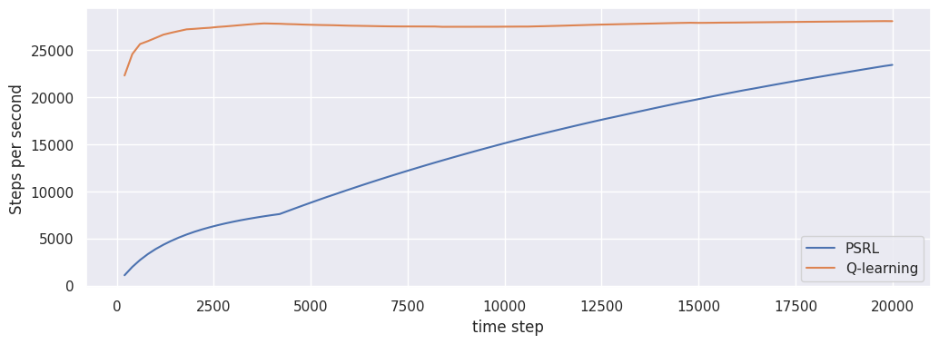
The \(\texttt{steps_per_second}\) indicators measures the average number of time steps per second.

The list of indicators can be obtained by calling the get_available_indicators function.

Available agents

Tabular episodic agents

PSRLEpisodic
QLearningEpisodic

Tabular continuous agents

PSRLContinuous
QLearningContinuous
UCRL2Continuous

Non-tabular episodic agents

ActorCriticEpisodic
ActorCriticRNNEpisodic
BootDQNEpisodic
DQNEpisodic

Non-tabular continuous agents

ActorCriticContinuous
ActorCriticRNNContinuous
BootDQNContinuous
DQNContinuous

Available MDP classes

DeepSea
FrozenLake
MiniGridEmpty
MiniGridRooms
RiverSwim
SimpleGrid
Taxi

Fixed MDP comparison

We compare QLearningEpisodic with PSRLEpisodic in RiverSwimEpisodic for a total of \(20\ 000\) time steps. As the MDP is fixed, we can compare the performances without necessarily using the normalized versions of the indicators.

seed = 42
optimization_horizon = 20_000
log_every=200

# Instantiate the MDP
mdp = RiverSwimEpisodic(seed=0, size=4, p_rand=0.01)

# Instantiate the agents
q_learning_agent = QLearningEpisodic(
    mdp_specs=make_mdp_spec(mdp),
    seed=seed,
    optimization_horizon=optimization_horizon,
    c_1 = 0.95,
    p = 0.05
)
psrl_agent = PSRLEpisodic(
    mdp_specs=make_mdp_spec(mdp),
    seed=seed,
    optimization_horizon=optimization_horizon,
)

# q-learning  interaction
loop_ql = MDPLoop(mdp, q_learning_agent)
loop_ql.run(T=optimization_horizon, log_every=log_every)

# PSRL interaction
loop_psrl = MDPLoop(mdp, psrl_agent)
loop_psrl.run(T=optimization_horizon, log_every=log_every)

Cumulative reward

# Create the shared axis for the plot
fig, ax = plt.subplots(1, 1, figsize=(12, 4))

# Plot the cumulative reward of the q-learning agent without the baselines
loop_ql.plot("cumulative_reward", ax, baselines=[])

# Plot the cumulative reward of the PSRL agent, including the baselines this time
loop_psrl.plot("cumulative_reward", ax)

# Display the figure
glue("cumulative_reward", fig, display=False)

Cumulative expected reward

fig1, ax = plt.subplots(1, 1, figsize=(12, 4))
loop_ql.plot("cumulative_expected_reward", ax, baselines=[])
loop_psrl.plot("cumulative_expected_reward", ax)
glue("cumulative_expected_reward", fig1, display=False)

Cumulative regret

fig, ax = plt.subplots(1, 1, figsize=(12, 4))
loop_ql.plot("cumulative_regret", ax, baselines=[])
loop_psrl.plot("cumulative_regret", ax)
glue("cumulative_regret", fig, display=False)
plt.show()

Steps per second

fig, ax = plt.subplots(1, 1, figsize=(12, 4))
loop_psrl.plot("steps_per_second", ax)
loop_ql.plot("steps_per_second", ax)
glue("steps_per_second", fig, display=False)
plt.show()

Fixed agent class comparison

We compare QLearningEpisodic in two different instances of RiverSwimEpisodic for a total of \(20\ 000\) time steps. In this case, the use of the normalized versions of the indicators.

seed = 42
optimization_horizon = 20_000

# Instantiate the MDPs
mdp_short = RiverSwimEpisodic(seed=0, size=4, p_rand=0.01)
mdo_long = RiverSwimEpisodic(seed=0, size=10, p_rand=0.01)

# Instantiate the agent
agent_for_short = QLearningEpisodic(
    mdp_specs=make_mdp_spec(mdp_short),
    seed=seed,
    optimization_horizon=optimization_horizon,
    c_1 = 0.95,
    p = 0.05
)
agent_for_long = QLearningEpisodic(
    mdp_specs=make_mdp_spec(mdo_long),
    seed=seed,
    optimization_horizon=2000,
    c_1 = 0.95,
    p = 0.05
)

# Short Riverswim interaction
loop_short = MDPLoop(mdp_short, agent_for_short)
loop_short.run(T=optimization_horizon, log_every=200)

# Long Riverswim interaction
loop_long = MDPLoop(mdo_long, agent_for_long)
loop_long.run(T=optimization_horizon, log_every=200)

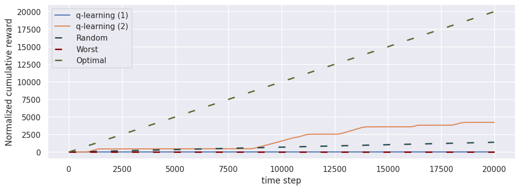
Normalized cumulative reward

fig, ax = plt.subplots(1, 1, figsize=(12, 4))
loop_long.plot("normalized_cumulative_reward", ax, label="q-learning (1)", baselines=[])
loop_short.plot("normalized_cumulative_reward", ax, label="q-learning (2)")
glue("normalized_cumulative_reward", fig, display=False)
plt.close()

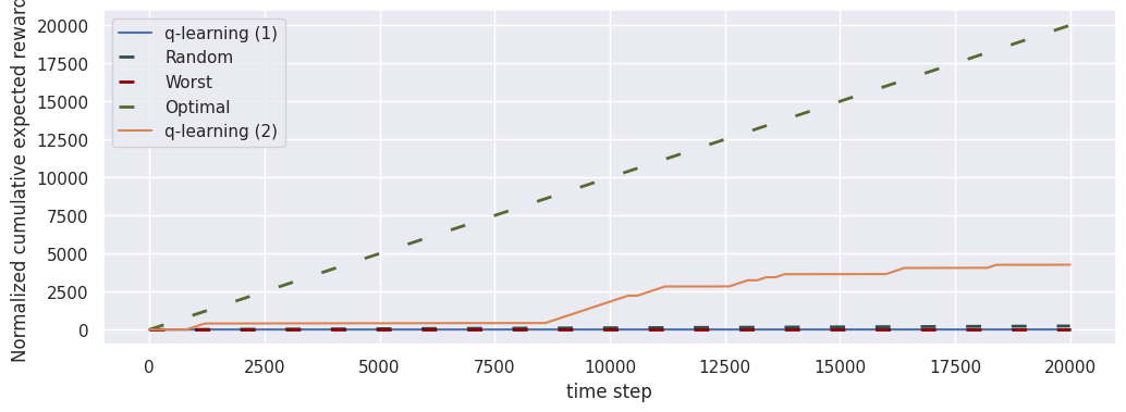
Normalized cumulative expected reward

fig, ax = plt.subplots(1, 1, figsize=(12, 4))
loop_long.plot("normalized_cumulative_expected_reward", ax, label="q-learning (1)")
loop_short.plot("normalized_cumulative_expected_reward", ax, label="q-learning (2)", baselines=[])
glue("normalized_cumulative_expected_reward", fig, display=False)
plt.close()

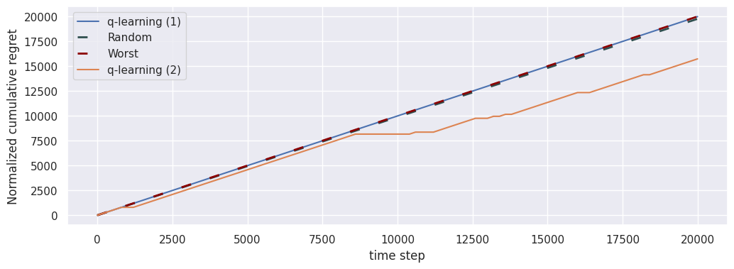
Normalized cumulative regret

fig, ax = plt.subplots(1, 1, figsize=(12, 4))
loop_long.plot("normalized_cumulative_regret", ax, label="q-learning (1)")
loop_short.plot("normalized_cumulative_regret", ax, label="q-learning (2)", baselines=[])
glue("normalized_cumulative_regret", fig, display=False)
plt.close()

Steps per second

fig, ax = plt.subplots(1, 1, figsize=(12, 4))
loop_long.plot("steps_per_second", ax, label="q-learning (1)")
loop_short.plot("steps_per_second", ax, label="q-learning (2)")
glue("normalized_steps_per_second", fig, display=False)
plt.close()