
Non-Tabular Benchmarking
Contents
Non-Tabular Benchmarking#
\(\texttt{Colosseum}\) is primarily developed for the tabular reinforcement learning setting. However, as our goal is to develop principled non-tabular benchmarks, we offer a way to test non-tabular reinforcement learning algorithms on the default \(\texttt{Colosseum}\) benchmark. Although our benchmark defines a challenge that is well characterized for tabular agents, we believe that it can provide valuable insights into the performance of non-tabular algorithms.
The BlockMDP model [Du et al., 2019] defines non-tabular versions of tabular MDPs. A BlockMDP is a tuple \(\left(\mathcal S, \mathcal A, P, P_0, R, \mathcal O, q\right)\), where \(\mathcal S\) is the tabular state space, \(\mathcal A\) is the action space, \(P\) is the transition kernel, \(P_0\) is the starting state distribution, \(R\) is the reward kernel, \(\mathcal O\) is the non-tabular observation space, and \(q : \mathcal S \to \Delta(\mathcal O)\) is a (possibly stochastic) emission map that associates a distribution over the observation space to each state in the MDP. Note that the agent is not provided with any information on the state space \(\mathcal S\).
Six deterministic emission maps are available. We present them below for the
SimpleGridContinuous MDP class.
One-hot encoding
The OneHotEncoding emission map assigns
to each state a feature vector that is filled with zeros except for an index that uniquely corresponds to the state.
mdp = SimpleGridContinuous(seed=42, size=4, emission_map=OneHotEncoding)
ts = mdp.reset()

print("Observation for the OneHotEncoding emission map.")
print(ts.observation)
Observation for the OneHotEncoding emission map.
[[1. 0. 0. 0. 0. 0. 0. 0. 0. 0. 0. 0. 0. 0. 0. 0.]]
Linear optimal value
The StateLinearOptimal
emission map assigns to each state a feature vector \(\phi(s)\) that enables linear representation of the optimal value
function. In other words, there is a \(\theta\) such that \(V^*(s) = \theta^T\phi(s)\).
mdp = SimpleGridContinuous(seed=42, size=4, emission_map=StateLinearOptimal)
ts = mdp.reset()

print("Observation for the StateLinearOptimal emission map.")
print(ts.observation.round(2))
Observation for the StateLinearOptimal emission map.
[[ 0.25  0.64  0.37 -0.11 -0.27  0.23  0.53 -0.07 -0.6  -0.08]]
Linear random value
The StateLinearRandom
emission map assigns to each state a feature vector \(\phi(s)\) that enables linear representation of the value function
of the randomly acting policy. In other words, there is a \(\theta\) such that \(V^\pi(s) = \theta^T\phi(s)\), where \(\pi\)
is the randomly acting policy.
mdp = SimpleGridContinuous(seed=42, size=4, emission_map=StateLinearRandom)
ts = mdp.reset()

print("Observation for the StateLinearRandom emission map.")
print(ts.observation.round(2))
Observation for the StateLinearRandom emission map.
[[ 0.25 -0.19  0.03  0.18 -0.06  0.09  0.39 -0.08 -0.19  0.29]]
Before presenting the StateInfo, ImageEncoding, and TensorEncoding emission maps, we review the textual
representation of the SimpleGridContinuous, which is used by those emission maps.
mdp = SimpleGridContinuous(seed=42, size=4)
mdp.reset()
print("Textual representation.")
print(mdp.get_grid_representation(mdp.cur_node))
Textual representation.
[['+' ' ' ' ' '-']
 [' ' 'A' ' ' ' ']
 [' ' ' ' ' ' ' ']
 ['-' ' ' ' ' '+']]
The letter A encodes the position of the agent and the symbols \(+\) and \(-\) represent the states that yield large reward and zero reward.
State information
The StateInfo emission map assigns to each state
a feature vector that contains uniquely identifying information about the state (e.g., coordinates for the DeepSea family).
mdp = SimpleGridContinuous(seed=42, size=4, emission_map=StateInfo)
ts = mdp.reset()

print("Observation for the StateInfo emission map.")
print(ts.observation)
Observation for the StateInfo emission map.
[[1. 2.]]
The observation vector corresponds to the x and y coordinates of the position of the agent.
Image encoding
The ImageEncoding emission map assigns to
each state a feature vector that contains uniquely identifying information about the state (e.g., coordinates for the
DeepSea mdp class).
mdp = SimpleGridContinuous(seed=42, size=4, emission_map=ImageEncoding)
ts = mdp.reset()

print("Observation for the ImageEncoding emission map.")
print(ts.observation)
Observation for the ImageEncoding emission map.
[[[2. 0. 0. 3.]
  [0. 1. 0. 0.]
  [0. 0. 0. 0.]
  [3. 0. 0. 2.]]]
In the observation matrix, \(1\) corresponds to the position of the agent, \(2\) to positive rewarding states, and \(3\) to non-rewarding states. The rest of the matrix is filled with zeros.
Tensor encoding
The TensorEncoding emission map assigns
to each state a tensor composed of the concatenation of matrices that one-hot encode the presence of a symbol in the
corresponding indices. For example, for the DeepSea family, the tensor is composed of a matrix that encodes the position
of the agent and a matrix that encodes the positions of white spaces.
mdp = SimpleGridContinuous(seed=42, size=4, emission_map=TensorEncoding)
ts = mdp.reset()

print("Observation for the TensorEncoding emission map.")
print(ts.observation)
Observation for the TensorEncoding emission map.
[[[[0. 0. 1. 0.]
   [1. 0. 0. 0.]
   [1. 0. 0. 0.]
   [0. 0. 0. 1.]]

  [[1. 0. 0. 0.]
   [0. 1. 0. 0.]
   [1. 0. 0. 0.]
   [1. 0. 0. 0.]]

  [[1. 0. 0. 0.]
   [1. 0. 0. 0.]
   [1. 0. 0. 0.]
   [1. 0. 0. 0.]]

  [[0. 0. 0. 1.]
   [1. 0. 0. 0.]
   [1. 0. 0. 0.]
   [0. 0. 1. 0.]]]]
Similarly to the ImageEncoding emission map, each element of the textual representation is encoded differently. In the TensorEncoding emission map, a one-hot encoding is used.
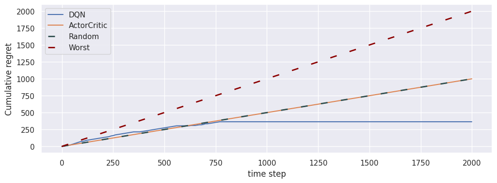
Non-tabular agent/MDP interactions#
Analysing the performances of non-tabular agents follows the same API of the tabular case. We present an example below.
seed = 1
optimization_horizon = 2_000

# Instantiate the MDP
mdp = SimpleGridContinuous(seed=42, size=4, emission_map=TensorEncoding)

# DQN
boot_dqn = DQNContinuous(
    seed=seed,
    mdp_specs=make_mdp_spec(mdp),
    optimization_horizon=optimization_horizon,
    **sample_agent_hyperparameters(DQNContinuous, seed),
)

# Perform the agent/MDP interaction
loop_dqn = MDPLoop(mdp, boot_dqn)
loop_dqn.run(T=optimization_horizon, log_every=10)

# ActorCritic
actor_critic = ActorCriticContinuous(
    mdp_specs=make_mdp_spec(mdp),
    seed=seed,
    optimization_horizon=optimization_horizon,
    **sample_agent_hyperparameters(ActorCriticContinuous, seed),
)
loop_ac = MDPLoop(mdp, actor_critic)
loop_ac.run(T=optimization_horizon, log_every=10)

# Plot the cumulative regret of the agents
fig, ax = plt.subplots(1, 1, figsize=(12, 4))
loop_dqn.plot(ax=ax, baselines=[])
loop_ac.plot(ax=ax)
plt.show()
Non-tabular hyperparameters optimization and benchmarking#
Similarly, the hyperparameters optimization and benchmarking procedures for the non-tabular setting can be carried out in the exact same way as for the tabular case.
In order to obtain the default \(\texttt{Colosseum}\) benchmarks, it is only required to set non_tabular=True when calling the
get_benchmark function as shown below.
ColosseumDefaultBenchmark.CONTINUOUS_ERGODIC.get_benchmark(
    "non_tabular_ce", non_tabular=True
)
- DKJ+19
Simon Du, Akshay Krishnamurthy, Nan Jiang, Alekh Agarwal, Miroslav Dudik, and John Langford. Provably efficient RL with rich observations via latent state decoding. In International Conference on Machine Learning, 1665–1674. PMLR, 2019.