Empirical hardness analysis
Empirical hardness analysis#
Measuring and understanding the hardness of MDPs represent a fundamental step in the development of a reinforcement learning benchmark. This tutorial introduces the hardness measures available in \(\texttt{Colosseum}\) and illustrates how to carry out the empirical analysis presented in the paper for the measures available in the package and for custom ones.
Measures of hardness
The three efficiently computable theoretical measures of hardness available are the diameter, the environmental value norm, and the sum of the reciprocals of the sub-optimality gaps.
Their code names can be obtained from the
get_available_hardness_measures
function.
There are two ways to compute the measures for a
BaseMDP
object.
You can either call the corresponding properties,
diameter,
value_norm, and
sum_reciprocals_suboptimality_gaps,
or alternatively you can use the
get_measure_from_name
function, which takes the code name of the measure as input.
mdp = SimpleGridContinuous(seed=0, size=4, p_rand=0.01, n_starting_states=3)
mdp.diameter
Diameter: 6.05
mdp.value_norm
Environmental value norm: 0.50
mdp.sum_reciprocals_suboptimality_gaps
Sum of the reciprocals of the suboptimality gaps: 361.30
Or alternatively,
mdp = SimpleGridContinuous(seed=0, size=4, p_rand=0.01, n_starting_states=3)
for measure_name in BaseMDP.get_available_hardness_measures():
    print(f"{measure_name}: {mdp.get_measure_from_name(measure_name):.2f}")
diameter: 6.05
value_norm: 0.50
suboptimal_gaps: 361.30
Hardness scenarios
The accompanying paper proposes four scenarios to analyse the two different types of identified complexities: the visitation complexity, which relates to the difficulty of visiting all the states, and the estimation complexity, which relates to the discrepancy between the optimal policy and the best policy an agent can derive from a given estimate of the transition and reward kernels.
To define a scenario, we create a
HardnessAnalysisParams
object, which encodes the configurations for the scenario.
The run_scenario_analysis function runs a HardnessAnalysisParams and produces the corresponding figure.
Note the run_scenario_analysis is built on top of the get_varying_parameter_dfs, which computes the hardness measures for the MDP instances.
If multiprocessing is enabled get_varying_parameter_dfs will use multiple cores.
The SimpleGridContinuous class is used as a running example for the tutorial.
Scenario 1
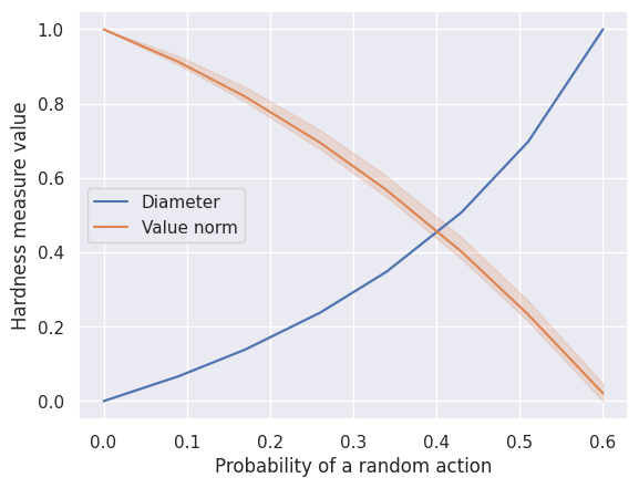
We vary the probability p_rand that an MDP executes a random action instead of the action selected by an agent. As p_rand approaches one, value estimation becomes easier, since outcomes depend less on agent choices. However, intentionally visiting states becomes harder.
SCENARIO_1_SimpleGridContinuous = HardnessAnalysisParams(
    mdp_class=SimpleGridContinuous,
    varying_params_name="p_rand",
    varying_params_name_clean="Probability of a random action",
    varying_params_values=np.linspace(0.0001, 0.6, 8).round(2),
    fixed_params=dict(make_reward_stochastic=True, size=8, n_starting_states=3),
    n_seeds_mdp=3,
)

run_scenario_analysis(SCENARIO_1_SimpleGridContinuous)
Scenario 2
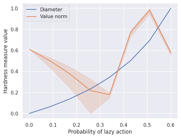
We vary the probability p_lazy that an MDP stays in the same state instead of executing
the action selected by an agent. Contrary to increasing p_rand, increasing p_lazy never benefits
exploration. Increasing p_lazy decreases estimation complexity and increases visitation complexity.
SCENARIO_2_SimpleGridContinuous = HardnessAnalysisParams(
    mdp_class=SimpleGridContinuous,
    varying_params_name="p_lazy",
    varying_params_name_clean="Probability of lazy action",
    varying_params_values=np.linspace(0.0001, 0.6, 8).round(2),
    fixed_params=dict(make_reward_stochastic=True, size=8, n_starting_states=3),
    n_seeds_mdp=3,
)

run_scenario_analysis(SCENARIO_2_SimpleGridContinuous)
Scenario 3
We vary the number of states across MDPs from the same family. Increasing the number of states simultaneously increases the estimation complexity and the visitation complexity.
SCENARIO_3_SimpleGridContinuous = HardnessAnalysisParams(
    mdp_class=SimpleGridContinuous,
    varying_params_name="size",
    varying_params_name_clean="Number of states",
    varying_params_values=np.arange(4, 12, 2),
    fixed_params=dict(make_reward_stochastic=True, n_starting_states=3),
    n_seeds_mdp=3,
)

run_scenario_analysis(SCENARIO_3_SimpleGridContinuous)
Scenario 4
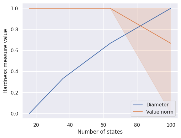
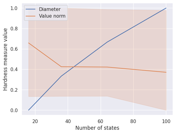
We vary the number of states across MDPs from the same family with a fixed value of p_rand = 0.1. Increasing the number of states simultaneously increases the estimation complexity and the visitation complexity.
SCENARIO_4_SimpleGridContinuous = HardnessAnalysisParams(
    mdp_class=SimpleGridContinuous,
    varying_params_name="size",
    varying_params_name_clean="Number of states",
    varying_params_values=np.arange(4, 12, 2),
    fixed_params=dict(make_reward_stochastic=True, p_rand=0.1, n_starting_states=3),
    n_seeds_mdp=3,
)

run_scenario_analysis(SCENARIO_4_SimpleGridContinuous)
Custom scenario
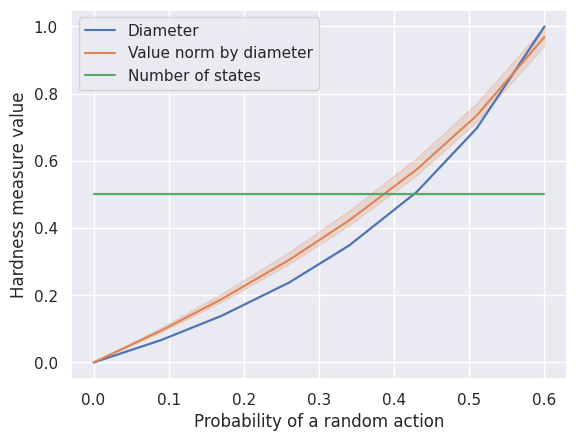
Running custom scenarios with custom measures of hardness is straightforward since it is possible to specify custom measures of hardness in the HardnessAnalysisParams configuration.
def number_of_states(mdp: BaseMDP) -> float:
    """
    A trivial measure of hardness that simply counts the number of states.
    """
    return mdp.n_states

def value_norm_by_diameter(mdp: BaseMDP) -> float:
    """
    A measure of hardness obtained by multiplying the diameter by the environmental value norm.
    """
    return mdp.diameter * mdp.value_norm

custom_scenario_SimpleGridContinuous = HardnessAnalysisParams(
    mdp_class=SimpleGridContinuous,
    varying_params_name="p_rand",
    varying_params_name_clean="Probability of a random action",
    varying_params_values=np.linspace(0.0001, 0.6, 8).round(2),
    fixed_params=dict(make_reward_stochastic=True, size=8, n_starting_states=3),
    hardness_measures=("diameter", value_norm_by_diameter, number_of_states),
    n_seeds_mdp=3,
)

run_scenario_analysis(custom_scenario_SimpleGridContinuous)
