
Inspect Markov Decision Processes
Inspect Markov Decision Processes#
The BaseMDP class efficiently computes important properties of the MDP.
This tutorial introduces some of them.
For the sake of the tutorial, we focus on the continuous setting.
Note however that a continuous MDP form such that the state space includes the in-episode time is available for every episodic MDP.
The API documentation of the EpisodicMDP class reports and describes the episodic-setting specific properties and functions.
Custom MDP
Before diving into the tutorial, we introduce the CustomMDP class, which can be used to instantiate an MDP from a transition kernel, a matrix of deterministic rewards (or a dictionary of random variables for stochastic rewards), and a starting state distribution.
Note that all the properties available for the BaseMDP class are also available for CustomMDP.
n_states = 4
n_actions = 2

### Transition kernel
T = [
  [
      [0.0, 1.0, 0.0, 0.0], # next state distribtion for selecting action 0 in state 0, i.e. T(0, 0)
      [0.0, 0.0, 1.0, 0.0], # next state distribtion for selecting action 1 in state 0, i.e. T(0, 1)
  ],
  [
      [0.0, 0.0, 0.5, 0.5], # next state distribution for selecting action 0 in state 1, i.e. T(1, 0)
      [0.0, 0.8, 0.1, 0.1], # next state distribution for selecting action 1 in state 1, i.e. T(1, 1)
  ],
  [
      [0.0, 0.5, 0.0, 0.5], # next state distribution for selecting action 0 in state 2, i.e. T(2, 0)
      [0.0, 0.1, 0.8, 0.1], # next state distribution for selecting action 1 in state 2, i.e. T(2, 1)
  ],
  [
      [0.5, 0.25, 0.25, 0.0], # next state distribution for selecting action 0 in state 3, i.e. T(3, 0)
      [0.1, 0.10, 0.10, 0.7], # next state distribution for selecting action 1 in state 3, i.e. T(3, 1)
  ],
]

### Reward distributions

# defined as a dictionary of scipy distributions
R = {
  (s, a): beta(np.random.uniform(0, 30), np.random.uniform(0, 30))
  for s in range(n_states)
  for a in range(n_actions)
}
# or as a matrix deterministic rewards
# R = np.random.randn(n_states, n_actions)

# Starting state distribution that assigns equal probability to state 0 and state 1
T_0 = {0: 0.5, 1 : 0.5}

# Instantiate the CustomEpisodic object
mdp_custom = CustomEpisodic(seed=42, T_0=T_0, T=np.array(T).astype(np.float32), R=R)
A SimpleGrid MDP is taken as a running example for the tutorial.
mdp = SimpleGridContinuous(seed=0, size=4, p_rand=0.01, n_starting_states=3)
In addition to the optimal policy, the random uniform policy, and the worst policy, which are pre-computed by the package, we’ll compute the MDP properties for a custom policy.
A continuous policy is an array of dimensionality number of states by number of actions such that each row defines a probability distribution over actions, whereas an episodic policy is an array of dimensionality episode length by number of states by number of action such that each in-episode time and state are associated with a probability distribution over actions.
pi = mdp._rng.dirichlet([1.0] * mdp.n_actions, mdp.n_states)
print("Continuous policy shape: ", pi.shape)
print(pi.round(2))
Continuous policy shape:  (16, 5)
[[0.5  0.   0.11 0.34 0.05]
 [0.28 0.02 0.09 0.01 0.6 ]
 [0.06 0.09 0.58 0.27 0.01]
 [0.04 0.19 0.17 0.05 0.54]
 [0.22 0.18 0.21 0.31 0.09]
 [0.1  0.05 0.04 0.56 0.26]
 [0.36 0.14 0.16 0.03 0.31]
 [0.17 0.53 0.21 0.09 0.01]
 [0.01 0.23 0.12 0.16 0.47]
 [0.74 0.04 0.17 0.05 0.  ]
 [0.29 0.08 0.1  0.18 0.36]
 [0.19 0.4  0.06 0.31 0.04]
 [0.35 0.13 0.03 0.34 0.15]
 [0.19 0.16 0.48 0.02 0.15]
 [0.19 0.16 0.22 0.11 0.31]
 [0.47 0.03 0.17 0.03 0.3 ]]
MDP communication class
The communication_class property returns an MDPCommunicationClass object, which is a Python enumeration for the possible MDP communication classes.
mdp.communication_class.name
'ERGODIC'
Starting states distribution
The starting_state_distribution property returns a Numpy array containing the probability of the states being sampled as starting states.
ssd = mdp.starting_state_distribution.round(2)
print("Starting state distribution", ssd)
Starting state distribution [0.33 0.33 0.   0.   0.   0.   0.   0.33 0.   0.   0.   0.   0.   0.
 0.   0.  ]
Expected rewards matrix
The
R
property returns a number of states by number of actions Numpy array such that to each state \(s\) and action \(a\) is associated with the expected reward following selecting \(a\) from \(s\).
We can visualise the matrix as a Pandas DataFrame.
pd.DataFrame(
    mdp.R.round(2),
    pd.Index(range(mdp.n_states), name="State"),
    pd.Index(map(lambda x: x.name, mdp.get_action_class()), name="Action"),
).style.set_table_attributes('style="font-size: 10px"')
| Action | UP | RIGHT | DOWN | LEFT | NO_OP |
|---|---|---|---|---|---|
| State | |||||
| 0 | 0.500000 | 0.500000 | 0.500000 | 0.500000 | 0.500000 |
| 1 | 0.500000 | 0.500000 | 0.500000 | 0.500000 | 0.500000 |
| 2 | 0.500000 | 0.500000 | 0.500000 | 0.500000 | 0.500000 |
| 3 | 0.500000 | 0.500000 | 0.500000 | 0.500000 | 0.500000 |
| 4 | 0.500000 | 0.500000 | 0.500000 | 0.500000 | 0.500000 |
| 5 | 0.500000 | 0.500000 | 0.500000 | 0.500000 | 0.500000 |
| 6 | 0.500000 | 0.500000 | 0.500000 | 0.500000 | 0.500000 |
| 7 | 0.500000 | 0.500000 | 0.500000 | 0.500000 | 0.500000 |
| 8 | 0.000000 | 0.500000 | 0.000000 | 0.500000 | 0.000000 |
| 9 | 0.500000 | 0.500000 | 0.500000 | 0.500000 | 0.500000 |
| 10 | 1.000000 | 0.500000 | 1.000000 | 1.000000 | 0.500000 |
| 11 | 0.500000 | 0.500000 | 0.500000 | 0.500000 | 0.500000 |
| 12 | 0.500000 | 0.000000 | 0.500000 | 0.000000 | 0.000000 |
| 13 | 0.500000 | 0.500000 | 0.500000 | 0.500000 | 0.500000 |
| 14 | 0.500000 | 0.500000 | 0.500000 | 0.500000 | 0.500000 |
| 15 | 0.500000 | 1.000000 | 0.500000 | 1.000000 | 1.000000 |
Transition kernel
The
T
property returns a number of states by number of actions by number of states Numpy array such that to each state \(s\) and action \(a\) is associated the probability distribution of the next state when selecting \(a\) from \(s\).
We can visualise the kernel using a Pandas DataFrame.
df = pd.MultiIndex.from_product(
    [
        range(mdp.n_states),
        map(lambda x: x.name, mdp.get_action_class()),
        range(mdp.n_states),
    ],
    names=["State from", "Action", "State to"],
)
df = pd.DataFrame(mdp.T.round(2).flatten(), index=df)
df = df.unstack(level="State to")
df.style.format(precision=2).set_table_attributes('style="font-size: 10px"')
| 0 | |||||||||||||||||
|---|---|---|---|---|---|---|---|---|---|---|---|---|---|---|---|---|---|
| State to | 0 | 1 | 2 | 3 | 4 | 5 | 6 | 7 | 8 | 9 | 10 | 11 | 12 | 13 | 14 | 15 | |
| State from | Action | ||||||||||||||||
| 0 | DOWN | 0.00 | 0.00 | 0.00 | 0.00 | 0.99 | 0.00 | 0.00 | 0.00 | 0.00 | 0.00 | 0.00 | 0.00 | 0.00 | 0.00 | 0.00 | 0.00 |
| LEFT | 0.99 | 0.00 | 0.00 | 0.00 | 0.00 | 0.00 | 0.00 | 0.00 | 0.00 | 0.00 | 0.00 | 0.00 | 0.00 | 0.00 | 0.00 | 0.00 | |
| NO_OP | 0.00 | 0.99 | 0.00 | 0.00 | 0.00 | 0.00 | 0.00 | 0.00 | 0.00 | 0.00 | 0.00 | 0.00 | 0.00 | 0.00 | 0.00 | 0.00 | |
| RIGHT | 0.00 | 0.00 | 0.99 | 0.00 | 0.00 | 0.00 | 0.00 | 0.00 | 0.00 | 0.00 | 0.00 | 0.00 | 0.00 | 0.00 | 0.00 | 0.00 | |
| UP | 0.00 | 0.00 | 0.00 | 0.99 | 0.00 | 0.00 | 0.00 | 0.00 | 0.00 | 0.00 | 0.00 | 0.00 | 0.00 | 0.00 | 0.00 | 0.00 | |
| 1 | DOWN | 0.99 | 0.00 | 0.00 | 0.00 | 0.00 | 0.00 | 0.00 | 0.00 | 0.00 | 0.00 | 0.00 | 0.00 | 0.00 | 0.00 | 0.00 | 0.00 |
| LEFT | 0.00 | 0.99 | 0.00 | 0.00 | 0.00 | 0.00 | 0.00 | 0.00 | 0.00 | 0.00 | 0.00 | 0.00 | 0.00 | 0.00 | 0.00 | 0.00 | |
| NO_OP | 0.00 | 0.00 | 0.00 | 0.00 | 0.00 | 0.99 | 0.00 | 0.00 | 0.00 | 0.00 | 0.00 | 0.00 | 0.00 | 0.00 | 0.00 | 0.00 | |
| RIGHT | 0.00 | 0.00 | 0.00 | 0.00 | 0.00 | 0.00 | 0.99 | 0.00 | 0.00 | 0.00 | 0.00 | 0.00 | 0.00 | 0.00 | 0.00 | 0.00 | |
| UP | 0.00 | 0.00 | 0.00 | 0.00 | 0.00 | 0.00 | 0.00 | 0.99 | 0.00 | 0.00 | 0.00 | 0.00 | 0.00 | 0.00 | 0.00 | 0.00 | |
| 2 | DOWN | 0.00 | 0.00 | 0.00 | 0.00 | 0.00 | 0.00 | 0.00 | 0.00 | 0.00 | 0.00 | 0.99 | 0.00 | 0.00 | 0.00 | 0.00 | 0.00 |
| LEFT | 0.99 | 0.00 | 0.00 | 0.00 | 0.00 | 0.00 | 0.00 | 0.00 | 0.00 | 0.00 | 0.00 | 0.00 | 0.00 | 0.00 | 0.00 | 0.00 | |
| NO_OP | 0.00 | 0.00 | 0.00 | 0.00 | 0.00 | 0.00 | 0.99 | 0.00 | 0.00 | 0.00 | 0.00 | 0.00 | 0.00 | 0.00 | 0.00 | 0.00 | |
| RIGHT | 0.00 | 0.00 | 0.99 | 0.00 | 0.00 | 0.00 | 0.00 | 0.00 | 0.00 | 0.00 | 0.00 | 0.00 | 0.00 | 0.00 | 0.00 | 0.00 | |
| UP | 0.00 | 0.00 | 0.99 | 0.00 | 0.00 | 0.00 | 0.00 | 0.00 | 0.00 | 0.00 | 0.00 | 0.00 | 0.00 | 0.00 | 0.00 | 0.00 | |
| 3 | DOWN | 0.00 | 0.00 | 0.00 | 0.99 | 0.00 | 0.00 | 0.00 | 0.00 | 0.00 | 0.00 | 0.00 | 0.00 | 0.00 | 0.00 | 0.00 | 0.00 |
| LEFT | 0.99 | 0.00 | 0.00 | 0.00 | 0.00 | 0.00 | 0.00 | 0.00 | 0.00 | 0.00 | 0.00 | 0.00 | 0.00 | 0.00 | 0.00 | 0.00 | |
| NO_OP | 0.00 | 0.00 | 0.00 | 0.00 | 0.00 | 0.00 | 0.00 | 0.00 | 0.00 | 0.00 | 0.00 | 0.99 | 0.00 | 0.00 | 0.00 | 0.00 | |
| RIGHT | 0.00 | 0.00 | 0.00 | 0.99 | 0.00 | 0.00 | 0.00 | 0.00 | 0.00 | 0.00 | 0.00 | 0.00 | 0.00 | 0.00 | 0.00 | 0.00 | |
| UP | 0.00 | 0.00 | 0.00 | 0.00 | 0.00 | 0.00 | 0.00 | 0.00 | 0.00 | 0.00 | 0.99 | 0.00 | 0.00 | 0.00 | 0.00 | 0.00 | |
| 4 | DOWN | 0.00 | 0.00 | 0.00 | 0.00 | 0.99 | 0.00 | 0.00 | 0.00 | 0.00 | 0.00 | 0.00 | 0.00 | 0.00 | 0.00 | 0.00 | 0.00 |
| LEFT | 0.00 | 0.00 | 0.00 | 0.00 | 0.00 | 0.00 | 0.00 | 0.99 | 0.00 | 0.00 | 0.00 | 0.00 | 0.00 | 0.00 | 0.00 | 0.00 | |
| NO_OP | 0.99 | 0.00 | 0.00 | 0.00 | 0.00 | 0.00 | 0.00 | 0.00 | 0.00 | 0.00 | 0.00 | 0.00 | 0.00 | 0.00 | 0.00 | 0.00 | |
| RIGHT | 0.00 | 0.00 | 0.00 | 0.00 | 0.00 | 0.00 | 0.00 | 0.00 | 0.00 | 0.00 | 0.00 | 0.99 | 0.00 | 0.00 | 0.00 | 0.00 | |
| UP | 0.00 | 0.00 | 0.00 | 0.00 | 0.00 | 0.00 | 0.00 | 0.00 | 0.00 | 0.00 | 0.00 | 0.00 | 0.00 | 0.99 | 0.00 | 0.00 | |
| 5 | DOWN | 0.00 | 0.00 | 0.00 | 0.00 | 0.00 | 0.00 | 0.00 | 0.00 | 0.00 | 0.99 | 0.00 | 0.00 | 0.00 | 0.00 | 0.00 | 0.00 |
| LEFT | 0.00 | 0.99 | 0.00 | 0.00 | 0.00 | 0.00 | 0.00 | 0.00 | 0.00 | 0.00 | 0.00 | 0.00 | 0.00 | 0.00 | 0.00 | 0.00 | |
| NO_OP | 0.00 | 0.00 | 0.00 | 0.00 | 0.00 | 0.99 | 0.00 | 0.00 | 0.00 | 0.00 | 0.00 | 0.00 | 0.00 | 0.00 | 0.00 | 0.00 | |
| RIGHT | 0.00 | 0.00 | 0.00 | 0.00 | 0.00 | 0.99 | 0.00 | 0.00 | 0.00 | 0.00 | 0.00 | 0.00 | 0.00 | 0.00 | 0.00 | 0.00 | |
| UP | 0.00 | 0.00 | 0.00 | 0.00 | 0.00 | 0.00 | 0.00 | 0.00 | 0.99 | 0.00 | 0.00 | 0.00 | 0.00 | 0.00 | 0.00 | 0.00 | |
| 6 | DOWN | 0.00 | 0.00 | 0.00 | 0.00 | 0.00 | 0.00 | 0.99 | 0.00 | 0.00 | 0.00 | 0.00 | 0.00 | 0.00 | 0.00 | 0.00 | 0.00 |
| LEFT | 0.00 | 0.00 | 0.99 | 0.00 | 0.00 | 0.00 | 0.00 | 0.00 | 0.00 | 0.00 | 0.00 | 0.00 | 0.00 | 0.00 | 0.00 | 0.00 | |
| NO_OP | 0.00 | 0.00 | 0.00 | 0.00 | 0.00 | 0.00 | 0.99 | 0.00 | 0.00 | 0.00 | 0.00 | 0.00 | 0.00 | 0.00 | 0.00 | 0.00 | |
| RIGHT | 0.00 | 0.00 | 0.00 | 0.00 | 0.00 | 0.00 | 0.00 | 0.00 | 0.99 | 0.00 | 0.00 | 0.00 | 0.00 | 0.00 | 0.00 | 0.00 | |
| UP | 0.00 | 0.99 | 0.00 | 0.00 | 0.00 | 0.00 | 0.00 | 0.00 | 0.00 | 0.00 | 0.00 | 0.00 | 0.00 | 0.00 | 0.00 | 0.00 | |
| 7 | DOWN | 0.00 | 0.00 | 0.00 | 0.00 | 0.99 | 0.00 | 0.00 | 0.00 | 0.00 | 0.00 | 0.00 | 0.00 | 0.00 | 0.00 | 0.00 | 0.00 |
| LEFT | 0.00 | 0.00 | 0.00 | 0.00 | 0.00 | 0.00 | 0.00 | 0.00 | 0.00 | 0.00 | 0.00 | 0.00 | 0.00 | 0.00 | 0.99 | 0.00 | |
| NO_OP | 0.00 | 0.99 | 0.00 | 0.00 | 0.00 | 0.00 | 0.00 | 0.00 | 0.00 | 0.00 | 0.00 | 0.00 | 0.00 | 0.00 | 0.00 | 0.00 | |
| RIGHT | 0.00 | 0.00 | 0.00 | 0.00 | 0.00 | 0.00 | 0.00 | 0.99 | 0.00 | 0.00 | 0.00 | 0.00 | 0.00 | 0.00 | 0.00 | 0.00 | |
| UP | 0.00 | 0.00 | 0.00 | 0.00 | 0.00 | 0.00 | 0.00 | 0.00 | 0.00 | 0.99 | 0.00 | 0.00 | 0.00 | 0.00 | 0.00 | 0.00 | |
| 8 | DOWN | 0.00 | 0.00 | 0.00 | 0.00 | 0.00 | 0.00 | 0.00 | 0.00 | 1.00 | 0.00 | 0.00 | 0.00 | 0.00 | 0.00 | 0.00 | 0.00 |
| LEFT | 0.00 | 0.00 | 0.00 | 0.00 | 0.00 | 0.00 | 0.99 | 0.00 | 0.01 | 0.00 | 0.00 | 0.00 | 0.00 | 0.00 | 0.00 | 0.00 | |
| NO_OP | 0.00 | 0.00 | 0.00 | 0.00 | 0.00 | 0.00 | 0.00 | 0.00 | 1.00 | 0.00 | 0.00 | 0.00 | 0.00 | 0.00 | 0.00 | 0.00 | |
| RIGHT | 0.00 | 0.00 | 0.00 | 0.00 | 0.00 | 0.99 | 0.00 | 0.00 | 0.01 | 0.00 | 0.00 | 0.00 | 0.00 | 0.00 | 0.00 | 0.00 | |
| UP | 0.00 | 0.00 | 0.00 | 0.00 | 0.00 | 0.00 | 0.00 | 0.00 | 1.00 | 0.00 | 0.00 | 0.00 | 0.00 | 0.00 | 0.00 | 0.00 | |
| 9 | DOWN | 0.00 | 0.00 | 0.00 | 0.00 | 0.00 | 0.00 | 0.00 | 0.00 | 0.00 | 0.99 | 0.00 | 0.00 | 0.00 | 0.00 | 0.00 | 0.00 |
| LEFT | 0.00 | 0.00 | 0.00 | 0.00 | 0.00 | 0.99 | 0.00 | 0.00 | 0.00 | 0.00 | 0.00 | 0.00 | 0.00 | 0.00 | 0.00 | 0.00 | |
| NO_OP | 0.00 | 0.00 | 0.00 | 0.00 | 0.00 | 0.00 | 0.00 | 0.00 | 0.00 | 0.00 | 0.00 | 0.00 | 0.00 | 0.00 | 0.00 | 0.99 | |
| RIGHT | 0.00 | 0.00 | 0.00 | 0.00 | 0.00 | 0.00 | 0.00 | 0.00 | 0.00 | 0.99 | 0.00 | 0.00 | 0.00 | 0.00 | 0.00 | 0.00 | |
| UP | 0.00 | 0.00 | 0.00 | 0.00 | 0.00 | 0.00 | 0.00 | 0.99 | 0.00 | 0.00 | 0.00 | 0.00 | 0.00 | 0.00 | 0.00 | 0.00 | |
| 10 | DOWN | 0.00 | 0.00 | 0.00 | 0.00 | 0.00 | 0.00 | 0.00 | 0.00 | 0.00 | 0.00 | 1.00 | 0.00 | 0.00 | 0.00 | 0.00 | 0.00 |
| LEFT | 0.00 | 0.00 | 0.00 | 0.00 | 0.00 | 0.00 | 0.00 | 0.00 | 0.00 | 0.00 | 1.00 | 0.00 | 0.00 | 0.00 | 0.00 | 0.00 | |
| NO_OP | 0.00 | 0.00 | 0.00 | 0.99 | 0.00 | 0.00 | 0.00 | 0.00 | 0.00 | 0.00 | 0.01 | 0.00 | 0.00 | 0.00 | 0.00 | 0.00 | |
| RIGHT | 0.00 | 0.00 | 0.99 | 0.00 | 0.00 | 0.00 | 0.00 | 0.00 | 0.00 | 0.00 | 0.01 | 0.00 | 0.00 | 0.00 | 0.00 | 0.00 | |
| UP | 0.00 | 0.00 | 0.00 | 0.00 | 0.00 | 0.00 | 0.00 | 0.00 | 0.00 | 0.00 | 1.00 | 0.00 | 0.00 | 0.00 | 0.00 | 0.00 | |
| 11 | DOWN | 0.00 | 0.00 | 0.00 | 0.00 | 0.99 | 0.00 | 0.00 | 0.00 | 0.00 | 0.00 | 0.00 | 0.00 | 0.00 | 0.00 | 0.00 | 0.00 |
| LEFT | 0.00 | 0.00 | 0.00 | 0.00 | 0.00 | 0.00 | 0.00 | 0.00 | 0.00 | 0.00 | 0.00 | 0.99 | 0.00 | 0.00 | 0.00 | 0.00 | |
| NO_OP | 0.00 | 0.00 | 0.00 | 0.00 | 0.00 | 0.00 | 0.00 | 0.00 | 0.00 | 0.00 | 0.00 | 0.00 | 0.99 | 0.00 | 0.00 | 0.00 | |
| RIGHT | 0.00 | 0.00 | 0.00 | 0.99 | 0.00 | 0.00 | 0.00 | 0.00 | 0.00 | 0.00 | 0.00 | 0.00 | 0.00 | 0.00 | 0.00 | 0.00 | |
| UP | 0.00 | 0.00 | 0.00 | 0.00 | 0.00 | 0.00 | 0.00 | 0.00 | 0.00 | 0.00 | 0.00 | 0.99 | 0.00 | 0.00 | 0.00 | 0.00 | |
| 12 | DOWN | 0.00 | 0.00 | 0.00 | 0.00 | 0.00 | 0.00 | 0.00 | 0.00 | 0.00 | 0.00 | 0.00 | 0.00 | 0.01 | 0.99 | 0.00 | 0.00 |
| LEFT | 0.00 | 0.00 | 0.00 | 0.00 | 0.00 | 0.00 | 0.00 | 0.00 | 0.00 | 0.00 | 0.00 | 0.00 | 1.00 | 0.00 | 0.00 | 0.00 | |
| NO_OP | 0.00 | 0.00 | 0.00 | 0.00 | 0.00 | 0.00 | 0.00 | 0.00 | 0.00 | 0.00 | 0.00 | 0.00 | 1.00 | 0.00 | 0.00 | 0.00 | |
| RIGHT | 0.00 | 0.00 | 0.00 | 0.00 | 0.00 | 0.00 | 0.00 | 0.00 | 0.00 | 0.00 | 0.00 | 0.00 | 1.00 | 0.00 | 0.00 | 0.00 | |
| UP | 0.00 | 0.00 | 0.00 | 0.00 | 0.00 | 0.00 | 0.00 | 0.00 | 0.00 | 0.00 | 0.00 | 0.99 | 0.01 | 0.00 | 0.00 | 0.00 | |
| 13 | DOWN | 0.00 | 0.00 | 0.00 | 0.00 | 0.00 | 0.00 | 0.00 | 0.00 | 0.00 | 0.00 | 0.00 | 0.00 | 0.99 | 0.00 | 0.00 | 0.00 |
| LEFT | 0.00 | 0.00 | 0.00 | 0.00 | 0.00 | 0.00 | 0.00 | 0.00 | 0.00 | 0.00 | 0.00 | 0.00 | 0.00 | 0.99 | 0.00 | 0.00 | |
| NO_OP | 0.00 | 0.00 | 0.00 | 0.00 | 0.99 | 0.00 | 0.00 | 0.00 | 0.00 | 0.00 | 0.00 | 0.00 | 0.00 | 0.00 | 0.00 | 0.00 | |
| RIGHT | 0.00 | 0.00 | 0.00 | 0.00 | 0.00 | 0.00 | 0.00 | 0.00 | 0.00 | 0.00 | 0.00 | 0.00 | 0.00 | 0.99 | 0.00 | 0.00 | |
| UP | 0.00 | 0.00 | 0.00 | 0.00 | 0.00 | 0.00 | 0.00 | 0.00 | 0.00 | 0.00 | 0.00 | 0.00 | 0.00 | 0.00 | 0.99 | 0.00 | |
| 14 | DOWN | 0.00 | 0.00 | 0.00 | 0.00 | 0.00 | 0.00 | 0.00 | 0.00 | 0.00 | 0.00 | 0.00 | 0.00 | 0.00 | 0.00 | 0.99 | 0.00 |
| LEFT | 0.00 | 0.00 | 0.00 | 0.00 | 0.00 | 0.00 | 0.00 | 0.99 | 0.00 | 0.00 | 0.00 | 0.00 | 0.00 | 0.00 | 0.00 | 0.00 | |
| NO_OP | 0.00 | 0.00 | 0.00 | 0.00 | 0.00 | 0.00 | 0.00 | 0.00 | 0.00 | 0.00 | 0.00 | 0.00 | 0.00 | 0.99 | 0.00 | 0.00 | |
| RIGHT | 0.00 | 0.00 | 0.00 | 0.00 | 0.00 | 0.00 | 0.00 | 0.00 | 0.00 | 0.00 | 0.00 | 0.00 | 0.00 | 0.00 | 0.00 | 0.99 | |
| UP | 0.00 | 0.00 | 0.00 | 0.00 | 0.00 | 0.00 | 0.00 | 0.00 | 0.00 | 0.00 | 0.00 | 0.00 | 0.00 | 0.00 | 0.99 | 0.00 | |
| 15 | DOWN | 0.00 | 0.00 | 0.00 | 0.00 | 0.00 | 0.00 | 0.00 | 0.00 | 0.00 | 0.99 | 0.00 | 0.00 | 0.00 | 0.00 | 0.00 | 0.01 |
| LEFT | 0.00 | 0.00 | 0.00 | 0.00 | 0.00 | 0.00 | 0.00 | 0.00 | 0.00 | 0.00 | 0.00 | 0.00 | 0.00 | 0.00 | 0.00 | 1.00 | |
| NO_OP | 0.00 | 0.00 | 0.00 | 0.00 | 0.00 | 0.00 | 0.00 | 0.00 | 0.00 | 0.00 | 0.00 | 0.00 | 0.00 | 0.00 | 0.00 | 1.00 | |
| RIGHT | 0.00 | 0.00 | 0.00 | 0.00 | 0.00 | 0.00 | 0.00 | 0.00 | 0.00 | 0.00 | 0.00 | 0.00 | 0.00 | 0.00 | 0.00 | 1.00 | |
| UP | 0.00 | 0.00 | 0.00 | 0.00 | 0.00 | 0.00 | 0.00 | 0.00 | 0.00 | 0.00 | 0.00 | 0.00 | 0.00 | 0.00 | 0.99 | 0.01 | |
Stationary distribution
The
optimal_stationary_distribution
, the
worst_stationary_distribution
, and the
random_stationary_distribution
properties return Numpy arrays containing the stationary distributions of the Markov chain yielded by the optimal, worst, and uniformly random policies.
We can compute the stationary distribution associated with a custom policy using the
get_stationary_distribution
function.
osd = mdp.optimal_stationary_distribution.round(2)
wsd = mdp.worst_stationary_distribution.round(2)
rsd = mdp.random_stationary_distribution.round(2)
sd = mdp.get_stationary_distribution(pi).round(2)
osd_node_labels = mdp.get_node_labels(osd)
wsd_node_labels = mdp.get_node_labels(wsd)
rsd_node_labels = mdp.get_node_labels(rsd)
sd_node_labels = mdp.get_node_labels(sd)


fig1, ax = plt.subplots(1, 1, figsize=(6, 6))
nx.draw(
    mdp.G,
    mdp.graph_layout,
    labels=osd_node_labels,
    node_color="darkolivegreen",
    font_color="white",
    node_size=1500,
    ax=ax,
)
plt.tight_layout()
glue("osd", fig1)
plt.show()

fig2, ax = plt.subplots(1, 1, figsize=(6, 6))
nx.draw(
    mdp.G,
    mdp.graph_layout,
    labels=wsd_node_labels,
    node_color="darkred",
    font_color="white",
    node_size=1500,
    ax=ax,
)
glue("wsd", fig2)
plt.tight_layout()
plt.show()

fig3, ax = plt.subplots(1, 1, figsize=(6, 6))
nx.draw(
    mdp.G,
    mdp.graph_layout,
    labels=rsd_node_labels,
    node_color="darkslategray",
    font_color="white",
    node_size=1500,
    ax=ax,
)
glue("rsd", fig3)
plt.tight_layout()
plt.show()

fig4, ax = plt.subplots(1, 1, figsize=(6, 6))
nx.draw(
    mdp.G,
    mdp.graph_layout,
    labels=sd_node_labels,
    node_color="darkblue",
    font_color="white",
    node_size=1500,
    ax=ax,
)
plt.tight_layout()
glue("sd", fig4)
plt.show()
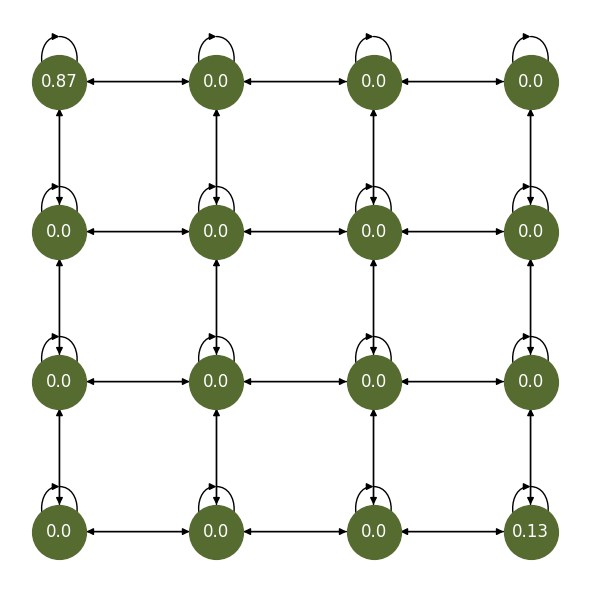
Fig. 1 The stationary distribution of the optimal policy.#
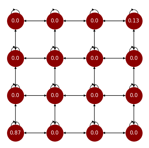
Fig. 2 The stationary distribution of the worst policy.#
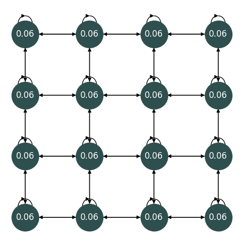
Fig. 3 The stationary distribution of the random policy.#
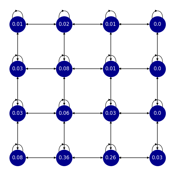
Fig. 4 The stationary distribution of a randomly sampled policy.#
Expected average reward
The
optimal_average_reward, the
worst_average_reward, and the
random_average_reward
properties return the expected time average reward, i.e.
\(
\underset{T\to \infty}{\text{lim inf}} \frac{1}{T} \mathbb{E}_\pi \sum_{t=0}^T R_t
\), associated to the optimal, worst, and uniformly random policies.
We can compute such measure for a custom policy using the
get_average_reward
function.
mdp.optimal_average_reward
mdp.worst_average_reward
mdp.random_average_reward
mdp.get_average_reward(pi)
Optimal policy |
Worst policy |
Random policy |
Randomly sampled policy |
|
|---|---|---|---|---|
Average regret |
0.996 |
0.004 |
0.500 |
0.484 |
Value functions
The
optimal_value_functions, the
worst_value_functions, and the
random_value_functions
properties return a tuple containing the state-action function and the state value function associated to the optimal, worst, and uniformly random policies.
We can compute the value function for a custom policy using the
get_value_functions
function.
ov = mdp.optimal_value_functions[1].round(2)
ov_node_labels = mdp.get_node_labels(ov)

wv = mdp.worst_value_functions[1].round(2)
wv_node_labels = mdp.get_node_labels(wv)

rv = mdp.random_value_functions[1].round(2)
rv_node_labels = mdp.get_node_labels(rv)

v = mdp.get_value_functions(pi)[1].round(2)
v_node_labels = mdp.get_node_labels(v)
fig, ax = plt.subplots(1, 1, figsize=(6, 6))
nx.draw(
    mdp.G,
    mdp.graph_layout,
    labels=ov_node_labels,
    node_color="darkolivegreen",
    font_color="white",
    node_size=1500,
    ax=ax,
    vmin = 0,
    vmax = 1
)
ax.set_title("Optimal value function")
glue("ov", fig)
plt.show()
#%%
fig, ax = plt.subplots(1, 1, figsize=(6, 6))
nx.draw(
    mdp.G,
    mdp.graph_layout,
    labels=wv_node_labels,
    node_color="darkred",
    font_color="white",
    node_size=1500,
    ax=ax,
)
ax.set_title("Value function of the worst policy")
plt.tight_layout()
glue("wv", fig)
plt.show()
#%%
fig, ax = plt.subplots(1, 1, figsize=(6, 6))
nx.draw(
    mdp.G,
    mdp.graph_layout,
    labels=rv_node_labels,
    node_color="darkslategray",
    font_color="white",
    node_size=1500,
    ax=ax,
)
ax.set_title("Value function of the random policy")
glue("rv", fig)
plt.show()
#%%
fig, ax = plt.subplots(1, 1, figsize=(6, 6))
nx.draw(
    mdp.G,
    mdp.graph_layout,
    labels=v_node_labels,
    node_color="darkblue",
    font_color="white",
    node_size=1500,
    ax=ax,
)
ax.set_title("Value function of a randomly sampled policy")
plt.tight_layout()
glue("v", fig)
plt.show()
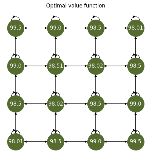
Fig. 5 The value function of the optimal policy.#
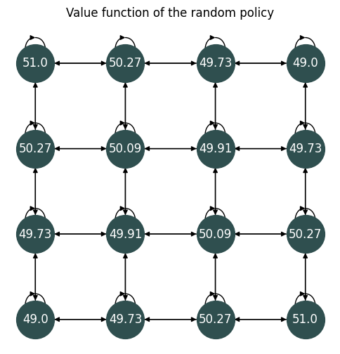
Fig. 6 The value function of the random policy.#
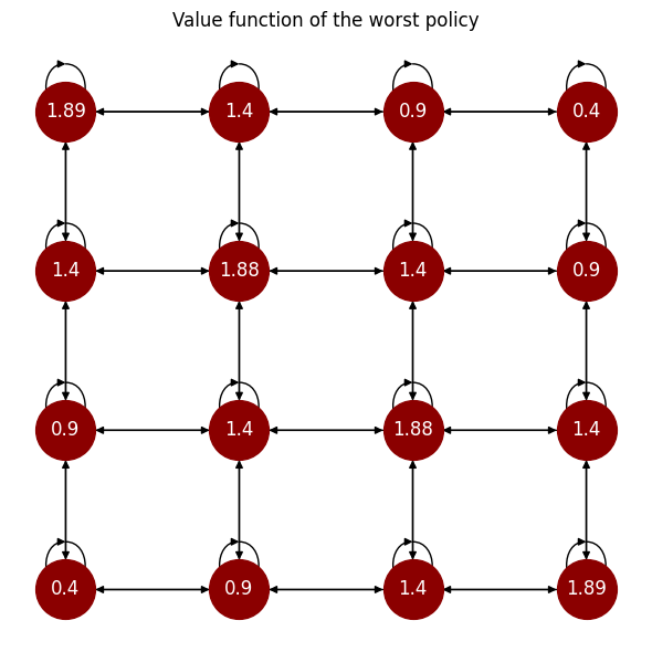
Fig. 7 The value function of the worst policy.#
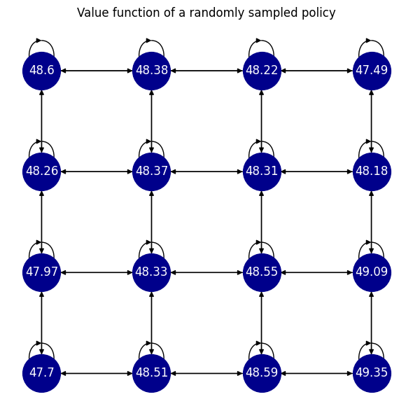
Fig. 8 The value function of a randomly sampled policy.#